Equivalent circuits of single-phase transformers
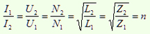
A. From Figure we take for the ideal transformers the basic equation:
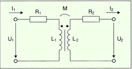
In Figure 9.3 you see the network of a transformer which corresponds to Fig. 9.1, where R
1, R
2 are the ohmic resistors of the wrappings and M is the mutual inductance between primary and secondary (see also Volume A, page 178). This circuit is applied to semitonal currents and voltages and as long as we accept even magnetic fields in the two legs of the magnetic circuit of the ferrite core. Figure also gives us:
U1 = (R1 + jωL1)I1 – jωM’I2’
U2 = jωM’I1 – (jωL2’ + R2’)I2’
The equations 9.2a, b include sizes open in the primary (those accented), that is they are transformed in connection with n. The sizes of the primary are not transformed, though the sizes of the secondary do. The opened sized are changing as following: the voltages are multiplied by n, R and L are multiplied by n2 and the currents are divided by n. Thus, we have: I2’=I2/n, U
2’=n∙U
2, L
2’=n
2∙L2, R
2’=n
2∙R
2 and M’=n∙M. In the same quadric-pole equations we notice that the transformation coefficient n is eliminated, which, on demand, can be taken as real (as now) or complex number. So, we can, on demand, design many equivalent circuits, as long as they correspond to the above quadric-pole equations.